Transformer / Encoder-Decoder Architecture
Notes on the Transformer architecture, including tokenization, embedding, positional encoding, encoder, decoder, and training.
Transformer / Encoder-Decoder Architecture
Based on the groundbreaking 2017 paper Attention is all you need by Vaswani et al.
Tokenization / De-tokenization
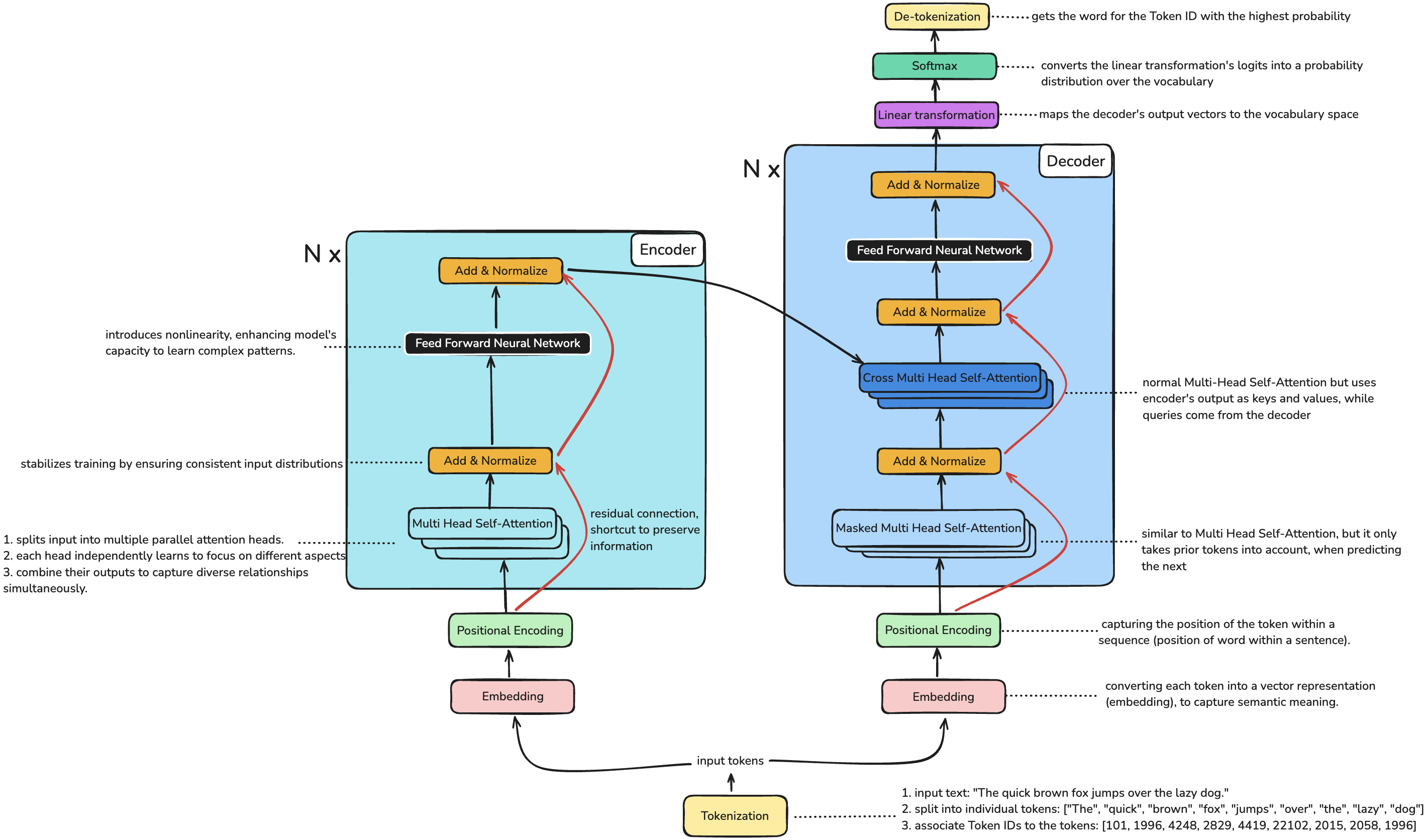
Tokenization is the process of associating an index with a token
- input text: "The quick brown fox jumps over the lazy dog."
- split into individual tokens: ["The", "quick", "brown", "fox", "jumps", "over", "the", "lazy", "dog"]
- associate Token IDs to the tokens: [101, 1996, 4248, 2829, 4419, 22102, 2015, 2058, 1996]
De-tokenization is the reverse process, where you convert token IDs back into human-readable tokens (words or subwords), basically looking ups IDs.
Additional Considerations (beyond the basic Transformer):
- Special Tokens: Models often include special tokens like [CLS] for classification and [SEP] for separating sequences during tokenization.
- Subword Tokenization: Models like BERT and GPT use subword tokenization to manage unknown words and reduce vocabulary size by splitting words into smaller parts.
- Vocabulary Size: The vocabulary size and token-to-ID mapping are specific to each model and its training dataset.
Embedding
Embedding is the process of converting each token into a vector representation (embedding).
The dimensions of these vectors are defined by the model architecture. (512-dimensional vector in the original Transformer model) These embeddings capture semantic information about the tokens, allowing the model to process and understand the input text.
| Word | Vector embedding (512 dimensions) |
|---|---|
| cat | [1.5, -0.4, 7.2, 19.6, 20.2, …] |
| dog | [1.7, -0.3, 6.9, 19.1, 21.1, …] |
| fish | [-5.2, 3.1, 0.2, 8.1, 3.5, …] |
| fisherman | [-4.9, 3.6, 0.9, 7.8, 3.6, …] |
| triangle | [60.1, -60.3, 10, -12.3, 9.2, …] |
| PS4 Remote | [81.6, -72.1, 16, -20.2, 102, …] |
The embedding layer is initialized with random vectors and learns meaningful word representations during training through backpropagation, where similar words (like 'cat' and 'dog') gradually develop similar vectors.
Positional Encoding
Positional Encoding is used to encode the position of the token within a sequence (position of word within a sentence)
Unlike the embedding layer, positional encodings are not trained - they are deterministically calculated using sinusoidal functions, with these formulas:
Even Dimensions:
Odd Dimensions:
where:
posis the position of the token in the sequence.iis the dimension index.d_modelis the dimensionality of the embeddings (e.g., 512 in the original Transformer model).
| Word | Vector Embedding (512 dimensions) | Positional Embedding | Final Input Embedding (Token Embedding + Positional Embedding) |
|---|---|---|---|
| cat | [1.5, -0.4, 7.2, 19.6, 20.2, …] | [-0.29, 0.57, -0.49, -0.49, -0.96, …] | [1.5-0.29, -0.4+0.57, 7.2-0.49, 19.6-0.49, 20.2-0.96, …] |
| dog | [1.7, -0.3, 6.9, 19.1, 21.1, …] | [0.43, -0.54, -0.42, -0.3, 0.93, …] | [1.7+0.43, -0.3-0.54, 6.9-0.42, 19.1-0.3, 21.1+0.93, …] |
| fish | [-5.2, 3.1, 0.2, 8.1, 3.5, …] | [0.62, 0.21, -0.05, -0.53, 0.17, …] | [-5.2+0.62, 3.1+0.21, 0.2-0.05, 8.1-0.53, 3.5+0.17, …] |
| fisherman | [-4.9, 3.6, 0.9, 7.8, 3.6, …] | [-0.58, 0.95, -0.76, -0.79, 0.21, …] | [-4.9-0.58, 3.6+0.95, 0.9-0.76, 7.8-0.79, 3.6+0.21, …] |
Encoder
The encoder consists of n identical layers (6 in original paper), each with a multi-head self-attention mechanism and a positionwise feed-forward network.
Residual connections and layer normalization are applied to each sub-layer.
Core Components and Mechanisms:
Input
  ↓
┌─────────────────────────────┐
│         Encoder Layer       │ ╮
├─────────────────────────────┤ │
│     Multi-Head Attention    │ │
│             ↓               │ │
│      Add & Normalize        │ │  x6
│             ↓               │ │  Layers
│       Feed Forward Net      │ │
│             ↓               │ │
│      Add & Normalize        │ │
└─────────────────────────────┘ ╯
             ↓
         Final Output
Multi-Head Self-Attention
Multiple attention heads allow the model to focus on different aspects (syntactic relationships, semantic similarities) of information simultaneously.
Multi-Head Self-Attention is a bi-directional process -> meaning that it considers context from both the left and right of a word when encoding its output embedding. (which therefore contains the context of the word)
- this makes encoders good at extracting meaningful information, they can understand the relationships and sequences
Scaled Dot-Product Attention          Multi-Head Attention

              ┌────────┐                   ┌────────┐
              │ MatMul │                   │ Linear │
              └────────┘                   └────────┘
               ↑     ↑                         ↑
      ┌─────────┐                         ┌─────────┐
      │ SoftMax │                         │ Concat  │
      └─────────┘                         └─────────┘
           ↑         ↑                         ↑
    ┌────────────┐                    ┌──────────────────┐
    │    Scale   │                    │   Scaled Dot-    │ h×
    └────────────┘                    │Product Attention │
           ↑         ↑                └──────────────────┘
     ┌───────────┐                        ↑    ↑    ↑
     │   MatMul  │                     ┌────┐┌────┐┌────┐
     └───────────┘                     │Lin ││Lin ││Lin │ h×
        ↑   ↑        ↑                 └────┘└────┘└────┘
        Q   K        V                    ↑    ↑    ↑
                                          V    K    Q
Multi-Head Attention mechanism:
Think of attention like looking up information in a database:
- Query (Q): What you're looking for
- Key (K): The index or label of stored information
- Value (V): The actual content/information to retrieve
-
Attention score between a query and key is computed as:
-
Apply softmax to get attention weights:
-
Attention = weighted sum of values:
Multi-Head Attention combines h parallel attention heads, where each head processes the input differently (to capture different aspects of information):
Where each head attention computes:
Add & Normalize
Layer Norm: Stabilizes training by ensuring consistent input distributions (by adjusting their scale and distribution) Residual: Creates shortcuts for gradient flow and preserves original information preventing the vanishing gradient problem.
Input X (TokenEmbedding + PositionalEncoding)
   ↓
output₁ = LayerNorm(X + MultiHead(Q,K,V))      // first add & norm after multi-head
   ↓
output₂ = LayerNorm(output₁ + FFNN(output₁))    // second add & norm after FFNN
where:
Xis the input (residual connection or skip connection adds the input directly to the output of a layer (𝑥 + 𝐹(𝑥))- LayerNorm normalizes across features:
Feed Forward Neural Network
Feed-Forward Network (FFN) processes each position independently through expansion (512→2048), ReLU activation, and projection (2048→512).
It introduces nonlinearity -> enhancing model's capacity to learn complex patterns.
Input(512) → Linear1(2048) → ReLU → Linear2(512) → Output(512)
Than Add & Normalize the FFNN output to stabilize it:
- output₂ = LayerNorm(output₁ + FFNN(output₁))
Decoder:
The decoder consists of n identical layers (6 in original paper) that process the encoder's output and previously generated tokens to produce the output sequence.
The Add & Norm and FFNN components are identical to the encoder. The key differences are:
- Masked Self-Attention instead of Self-Attention
- Additional Cross-Attention layer
- Three sub-layers instead of two
Core Components and Mechanisms:
Target Input
     ↓
┌──────────────────────────┐
│      Decoder Layer       │ ╮
├──────────────────────────┤ │
│  Masked Self-Attention   │ │
│           ↓              │ │
│    Add & Normalize       │ │
│           ↓              │ │  x6
│    Cross Attention       │ │  Layers
│           ↓              │ │
│    Add & Normalize       │ │
│           ↓              │ │
│     Feed Forward Net     │ │
│           ↓              │ │
│    Add & Normalize       │ │
└──────────────────────────┘ ╯
           ↓
       Final Output
Masked Multi-Head Self-Attention
Masked Multi-Head Self-Attention is identical to Multi-Head Self-Attention but adds a masking operation that prevents the decoder from looking at future tokens during training and inference.
how masking works in the decoder's self-attention:
| Position | Input Token | Can See | Masked Tokens | Attention Matrix | Available Context |
|---|---|---|---|---|---|
| 1 | "I" | [I] | [am, happy] | [0, -∞, -∞] | "I" |
| 2 | "am" | [I, am] | [happy] | [0, 0, -∞] | "I am" |
| 3 | "happy" | [I, am, happy] | [ ] | [0, 0, 0] | "I am happy" |
If applied before softmax, -∞ becomes 0, effectively preventing attention to future tokens.
Scaled Dot-Product Attention          Multi-Head Attention

              ┌────────┐                   ┌────────┐
              │ MatMul │                   │ Linear │
              └────────┘                   └────────┘
               ↑     ↑                         ↑
      ┌─────────┐                         ┌─────────┐
      │ SoftMax │                         │ Concat  │
      └─────────┘                         └─────────┘
           ↑         ↑                         ↑
    ┌────────────┐                    ┌──────────────────┐
    │    Mask    │                    │   Scaled Dot-    │ h×
    └────────────┘                    │Product Attention │
           ↑         ↑                └──────────────────┘
     ┌───────────┐                        ↑    ↑    ↑
     │   Scale   │                   ┌────┐┌────┐┌────┐
     └───────────┘                   │Lin ││Lin ││Lin │ h×
           ↑         ↑               └────┘└────┘└────┘
       ┌────────┐                        ↑    ↑    ↑
       │ MatMul │                        V    K    Q
       └────────┘
          ↑  ↑       ↑
          Q  K       V
Add & Normalize in the Decoder
Residual connections are also used in the decoder to ensure information persits.
Input Y (Target TokenEmbedding + PositionalEncoding)
   ↓
output₁ = LayerNorm(Y + MaskedMultiHead(Q,K,V))      // first add & norm after masked self-attention
   ↓
output₂ = LayerNorm(output₁ + CrossAttention(Q,K,V))  // second add & norm after cross-attention
   ↓
output₃ = LayerNorm(output₂ + FFNN(output₂))         // third add & norm after FFNN
Cross Multi-Head Self-Attention
Cross Attention is just normal Multi-Head Self-Attention but uses encoder's output as keys and values, while queries come from the decoder's previous layer. This allows the decoder to focus on relevant parts of the input sequence to generate each output token.
   Decoder (Queries)     Encoder (Keys, Values)
         ↓                      ↓
   "What to look for"    "Where to look & what to get"
Output generation
- Linear transformation maps the decoder's output vectors to the vocabulary space, allowing the model to assign probabilities to each token for text generation.
- Softmax function converts the linear transformation's logits into a probability distribution over the vocabulary, ensuring the probabilities sum to one for token selection.
- De-tokenization converts the token with the highest probability into word (by basically looking ups IDs).
Training
Training involves optimizing the model's parameters through backpropagation.
                    ┌─────────────────┐
                    │  Input Sequence │
                    └────────┬────────┘
                             ↓
┌───────────────────────────────────────────────┐
│               Teacher Forcing                 │
│  (Use actual target tokens during training)   │
└───────────────────────────────────────────────┘
                             ↓
┌───────────────────────────────────────────────┐
│             Forward Propagation               │
│    1. Encoder processes input sequence        │
│    2. Decoder generates output sequence       │
└───────────────────────────────────────────────┘
                             ↓
┌───────────────────────────────────────────────┐
│             Loss Calculation                  │
│    1. Compare with target sequence            │
│    2. Apply label smoothing                   │
└───────────────────────────────────────────────┘
                             ↓
┌───────────────────────────────────────────────┐
│           Backward Propagation                │
│    1. Calculate gradients                     │
│    2. Apply gradient clipping                 │
└───────────────────────────────────────────────┘
                             ↓
┌───────────────────────────────────────────────┐
│            Parameter Updates                  │
│    1. Apply Adam optimizer                    │
│    2. Update learning rate                    │
└───────────────────────────────────────────────┘
Loss Function
The primary loss function is the cross-entropy loss between predicted and actual token probabilities:
where:
- is the true probability (usually one-hot encoded)
- is the predicted probability
- is the vocabulary size
Optimizer
The Adam optimizer with custom learning rate scheduling is used:
where:
- is the model dimension (512 in original paper)
- is typically 4000 steps
Regularization Techniques
-
Label Smoothing (ε = 0.1):
- Prevents overconfidence by distributing small probability mass across all labels:
-
Dropout (rate = 0.1) applied to:
- Attention weights
- Hidden states between layers
- Embedding layers
Training Configurations
Key hyperparameters from the original paper:
| Parameter | Value |
|---|---|
| Batch Size | 25,000 tokens |
| Training Steps | 100,000 |
| Warmup Steps | 4,000 |
| Dropout Rate | 0.1 |
| Label Smoothing | 0.1 |
| Adam β₁ | 0.9 |
| Adam β₂ | 0.98 |
| Adam ε | 10⁻⁹ |
The encoder and decoder can be trained independently:
-
Encoder Training:
- Optimized for understanding and representation
- Can be pre-trained on large text corpora
- Uses masked language modeling objectives
-
Decoder Training:
- Optimized for generation
- Can be fine-tuned for specific tasks
- Uses autoregressive prediction objectives Both Encoder & Decoder can be trained seperatly and not have to share weights
- meaning Encoder can be optmized to understand text and Decoder optmized for generating text.
Inference
Beam search maintains k-best hypotheses at each decoding step, where k is the beam width (e.g., k=4 in original paper).
Simple Example (k=2): Input: "How are" Target: Generate next words
Step 1: First Token Probabilities
"How are" → [
  "you" (0.6),    ← Keep
  "they" (0.5),   ← Keep
  "we" (0.3),     ← Discard
  "the" (0.2)     ← Discard
]

Step 2: Expand Each Path
"How are you" → [               "How are they" → [
  "doing" (0.6 × 0.5),           "doing" (0.5 × 0.4),
  "feeling" (0.6 × 0.3),         "all" (0.5 × 0.3),
  "today" (0.6 × 0.2)            "now" (0.5 × 0.2)
]                              ]

Combined and Ranked:
1. "How are you doing"   (0.30)  ← Keep
2. "How are they doing" (0.20)   ← Keep
3. "How are you feeling" (0.18)  ← Discard
4. "How are they all"    (0.15)  ← Discard
Score calculation: For sequence Y given input X:
where:
- is the sequence probability
- is sequence length
- is length penalty (0.6 in original paper)
Without Length Penalty (α=0):
Favors shorter: "How are you"

With Length Penalty (α=0.6):
Balances length: "How are you doing"
The search continues until:
- EOS token generated
- Maximum length reached (input_length + 50)
- Early termination conditions met